Design Optimization Project
MSE 426: Introduction to Engineering Design Optimization
Submitted to:
Prof. Dr. Gary Wang
TA. Di Wu
By Colin Leitner
Executive Summary
This document is an excerpt from the original which contained two other optimization projects by different authors. This version includes only:
Optimizing the Neural Network of a Virtual Self-Driving Car
By Colin Leitner
This problem consists of a realistic controllable vehicle in a virtual environment. Three main components work together: a simulation, a neural network, and a genetic algorithm (GA). The goal of the car’s virtual driver is to navigate a course as far as possible without touching any objects or going too slowly. This project uses an idea called “NeuroEvolution” discussed in the article “Evolving Neural Networks through Augmenting Topologies”[1], except here, the network topology is fixed and only weightings are evolved.
fitness = distance travelled
Where the distance of a driver is determined by the performance of 45 neural network coefficients in the simulation. All physical distances in this project are measured in simulation pixels. The scale is about 20 pixels per real-world meter. The distance for one lap of the course is about 4000 pixels, and will be used to judge optimality.
Initially, incorporation of time was attempted with functions like:
fitness = (distance)^2 / time
This was tested, but created a problem. Encouraging shorter times encourages faster failure (collision). Really, cars that can navigate the furthest are desired. To solve this, the exponent of distance was raised to higher powers in attempt to emphasize it, but time became so insignificant that it was therefore removed altogether. Ideally, the best car should never crash, although this may be difficult to generate considering the high dimensionality and extreme non-linearity of design variables.
These are checked every step in the simulation. Whenever a constraint is violated, the test ends and the distance is recorded.
- The velocity of the car must never be < 0.000000001 pixels per frame.
- The front edge of the car must never intersect with any box of the course at any time.
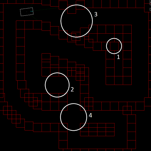
Figure 1: The view of a simulation in progress, rendered with OpenGL.
The simulation is a generalization of real driving conditions. Things that a car couldn’t cross (like road markings) or places it can’t go are all considered generic obstacles. The car exists as a simple white rectangle and a teal line pointing in the direction of its steering wheel. It has 4 basic controls: accelerate, brake, steer left, and steer right. These are designed emulate a real car. For example, the steering wheel position cannot be instantaneously moved, nor can the car instantly stop due to inertia.
To achieve the goal of staying in the lane and avoiding objects, only 3 distance sensors are used which radiate from the car. 3 was chosen because usually there's 3 ways to turn at an intersection. The real-world equivalent of these sensors would be laser radar. The distance sensors are shown as 3 green dotted lines.
In addition to the objective function, the course is specially designed to filter out drivers with bad practices. Some features are labelled in the image and are explained as follows:
Also, a variety of left and right turns of varying sharpness are included in the course to make sure that drivers do not become specialized on any one type of obstacle.
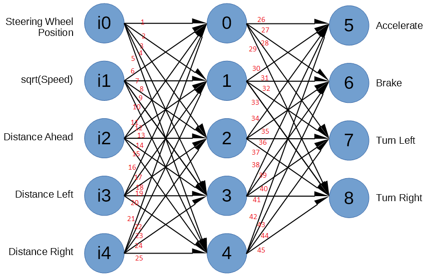
A "FeedForward" (meaning all links point one direction with no internal memory) artificial neural network (ANN) is evaluated in every step of the simulation to determine what actions the car should take based on its sensor inputs. The topology is fixed and can be visualized as seen in figure 2. The 45 link coefficients are what collectively defines a “driver”.
Figure 2: Topology of the ANN. Nodes with the letter i are input nodes
To evaluate the neural network, inputs are first all normalized to a value between 0-1. The square root of speed is used as input to make the ANN more precise at lower speeds. Then, from input nodes (marked with an i), the sensor value is multiplied by the weight of each link and added to a summation at the node each link points to. A link weight is a real value between -1 and 1. At each non-input node, each link weight is added to the sum only if the node they originate from is ON. Non-input nodes have a binary state: they turn ON only if the sum of the links pointing into it is > 0. No biasing of nodes is done; nodes rely solely on the value of other links to create their sum. Intermediate nodes are evaluated sequentially from 0-8, so that upstream nodes are calculated before ones downstream. Once all node states are known, the state of the last 4 nodes is copied to the controls of the car, which are then acted upon for one step of the simulation before reevaluating the ANN.
The number of nodes per intermediate layer (the center column of nodes in the figure) approximates how many scenarios a layer is able to distinguish from the previous layer. The number of layers (depth of the network) increases the non-linearity of the network. Sizing the ANN required a balance between enough freedom for the desired behaviour to be producible by the network, but small enough to be computationally cheap. Two layers were thought to provide enough non-linearity, and a width equal to the number of sensors was chosen. When connecting all nodes, this makes 45 link weights, each being a design variable that can be changed by the GA.They are numbered in the figure.
On its own, this ANN has no feedback or memory, since data only flows one way. This is solved by inputting the car’s speed and having an output of acceleration, and allowing the GA to naturally create feedback loops in the neural net. The same is done with the input of steering position and output of steering velocity. Not only does this allow feedback loops to arise organically in the net, but lets all systems dynamically interact with each other.
With the two previous components, the main problem becomes setting the coefficients of the ANN to make the car achieve a high objective function (distance through the course). A genetic algorithm (GA) is best suited to this problem because of the extreme multimodality of the objective function; non-optimal solutions must be considered and explored in order to avoid getting stuck on local minima. Tools like OASIS were also considered but interfacing the two programs would likely be a bottleneck in data transfer. Also, the two programs happened to exist on different OSs. Instead, a GA was written in C++ that can run inside the simulation. From the GA’s point of view, the array of 45 weights is the genome of one driver. First, to find starting points for the GA, approximately 10 million ANNs (drivers) with random coefficients were tested in the simulation over the course of several days. From these, the top 40 were chosen to form the population of the first generation.
Since two feasible neural networks could employ vastly different techniques, performing crossover would be no better than randomly generating a completely new set of coefficients. This happens because the same link in two different networks does not necessarily have the same role, and so swapping subsets of links does not swap subsets of driver features. The advantages of GA is still exploited by testing and storing many solutions in parallel and mutating non-optimal solutions to improve on them.
In the GA, rather than a conglomerated string of bits representing a driver’s genome, a vector of coefficients was used. This allows individual control on what gene to mutate and the magnitude. At the start, the chance of mutation per gene was set to 50%, and the max magnitude 0.2 to ensure the space of the design variables was thoroughly explored. The mutation magnitude is applied to the link weights in the range of -1 to 1. As drivers become more skilled, the chance of mutation was decreased to 20% and the max magnitude 0.01 to finely tune their behaviour. Other than the noted changes, the other features of the GA are standard, such as the number of children being proportional to fitness.
When replaying the results, the emergent behaviour of drivers can be studied. Some bad, yet feasible techniques were discovered such as “the right hand rule” where the driver seems to stay centered, but actually is just keeping a certain distance between itself and one wall, ignoring other walls. Drivers that zig-zag within the lane get higher scores because their path length is longer. There was some good strategies discovered too, such as initially turning the wrong direction when approaching a tight corner in order to take a wide smooth turn. The wider turns also helped drivers travel a longer distance.
The intersection proved to be difficult for drivers. Many hit the sharp corner of the intersection because their sensors could not see it. The intersection enabled drivers to turn any way they desired, and some turned around and headed back to the easier part of the course. To force drivers to complete full laps, the intersection was closed into a 90° bend for later tests.
From the initial population, it took an estimated 6,000 generations to produce a driver that could do a complete lap around the course, which was a distance of 3892 pixels. An exact generation number is not known because the output of sessions were repeatedly fed back into new sessions, while manually picking innovative drivers to speed up the process. Even the best drivers could not drive indefinitely around the track, which suggests that the techniques being used by most drivers are unstable, and sensitive to initial conditions.
In this project, the topology of the network was not eligible for evolution, but more complex algorithms are available to do this [1]. These keep track of the roles of links within the ANN and enable doing crossover.
Adding traffic light sensors and turn direction inputs to the ANN would allow controlling the direction the driver turns at an intersection. Also, with more distance sensors around the car, a higher-resolution understanding of surroundings would be available to the ANN.
The products of this project is an ANN and set of weights that performs the objective well in this configuration. Possible applications for these include:
[1] Kenneth O. Stanley & Risto Miikkulainen (2002). "Evolving Neural Networks Through Augmenting Topologies", The MIT Press, https://doi.org/10.1162/106365602320169811